fig 1. Animation of several different trusses being optimized

You can use Pytorch for more than just Neural Networks - its autograd is super powerful for any problem where you need gradients, but they’re hard to calculate manually.

The first step is solving a system of equations to find the force in each beam (edge) of the truss that balances each connection point (node). Finally, we sum up the “cost” of each of those edges, taking into account how strength changes with length and compression vs tension, etc.

Because we can write out the “cost” of a truss in closed form, we can use autograd to calculate its gradients, then use an optimizer to move the nodes to lower the cost.

The optimization transforms rigid, boxy truss designs into beautiful, organic curves. Check out the code on github.

Force calculation algorithm

Calculating all forces throughout the truss is done by solving a system of equations such that each node reaches equilibrium. For each node: the x and y components of all incoming force vectors exactly matches the load:

Take a equilateral triangle with a load of 10 applied downward at the top, and 5 applied up at each bottom

    A
   / \
  F1  F2
 /      \
B---F3---C

(A positive force is upward or rightward. Angles are relative to the horizontal)

Each node creates two equations, one for its X and one for its Y equilibrium:

Ax: F1*cos(th_ba) + F2*cos(th_ca) + 0             == -load_Ax (==0)
Ay: F1*sin(th_ba) + F2*sin(th_ca) + 0             == -load_Ay (==-10)
Bx: F1*cos(th_ab) + F2*0          + F3*cos(th_cb) == -load_Bx (==0)
By: F1*sin(th_ab) + F2*0          + F3*sin(th_cb) == -load_By (==5)
Cx: F1*0          + F2*cos(th_ac) + F3*cos(th_bc) == -load_Cx (==0)
Cy: F1*0          + F2*sin(th_ac) + F3*sin(th_bc) == -load_Cy (==5)

This can be written in matrix form as:

cos(th_ba), cos(th_ca), 0                     -load_Ax (==0)
sin(th_ba), sin(th_ca), 0              F1     -load_Ay (==-10)
cos(th_ab), 0         , cos(th_cb)  @  F2  == -load_Bx (==0)
sin(th_ab), 0         , sin(th_cb)     F3     -load_By (==5)
0         , cos(th_ac), cos(th_bc)            -load_Cx (==0)
0         , sin(th_ac), sin(th_bc)

A @ F = L

Where F is a vector of the forces in each beam, A is a matrix constructed from the x,y force equations for each node, and L is a vector of Loads. A will be 2N x M (x,y for each node) and M columns (one for each beam).

What about Anchor Points?

At an anchor point, any resultant force is allowed, because it is supplied by the anchor to the ground. A full anchor allows both X and Y forces to be non-zero, and a partial anchor allows a resulant force in just one dimension.

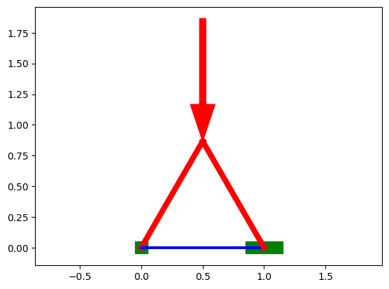
Fig 2. The right anchor point only constraints Y.

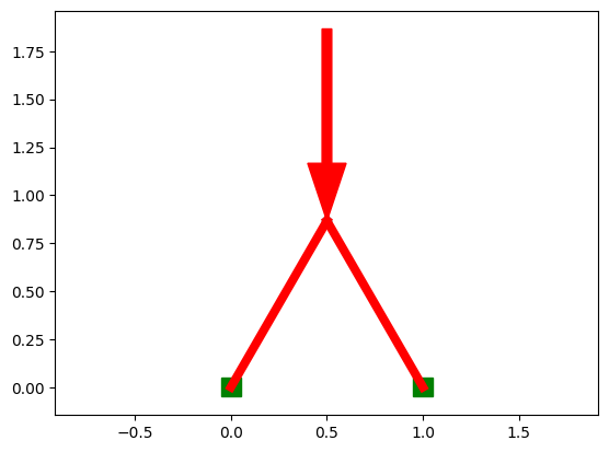
Fig 3. Both anchor points constrain X and Y.

Notice that the triangle with two full anchors does not need any tension in the bottom beam.

In order to account for anchor points, their nodes can simply be removed from the system of equations! A partial X or Y anchor can just have one of its two lines removed from the system.

Solving the Equation

Now we need to solve A @ F = L for our force vector F with torch.linalg.lstsq!

But will there always be a solution?

Underconstrained

If the system is underconstrained (Imagine a floating node with just a single edge), that means there will be some nodes that cannot reach equilibrium and will have a net force. Luckily, that is detected by the lstsq call, which will have a high residual! This will raise a ValueError when solving.

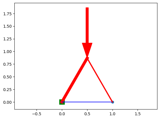
Fig 4. In an underconstrained system, some nodes cannot reach equilibrium.

Overconstrained systems

In an overconstrained system, there are many possible solutions of how force could be distributed among the beams. In reality, force would be distributed based on the stiffness and displacement of each beam. See this link for an example of solving this system more exactly.

Here, I’m simply letting the Least Squares solver minimize the L2 norm of the forces, which produces a decent result balancing the force between all the possible beams.

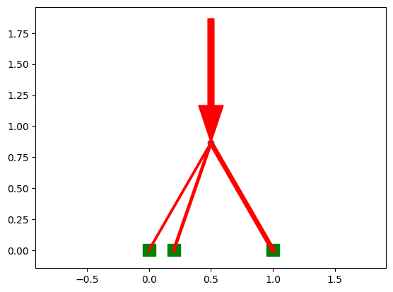
Fig 5. In an overconstrained system, there are many ways to split force among beams.

Optimizing the Truss

Here’s where the whole point of using pytorch comes in! Now that we’ve solved the force in each beam of the truss, we can calculate a total cost aka “loss” ;) and then move the nodes based on their gradient with respect to the total cost.

Tensile strength remains constant with length, but Compression strength gets weaker for longer beams because they risk bending and buckling.

Tension: cost = length * force / tensile_strength

Compression: cost = length * force / compression_strength(length)

We can set tensile_strength = 1 and use an approximation compression_strength = 3 / (length + 3) to get:

Compression: cost = length * force * (length + 3) / 3

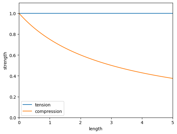
Fig 6. Graph of Compression and Tension strengths over distance. (No guarantees that this is realistic.)

Now we can sum up the costs of all the beams in compression and tension, backprop the gradients, and adjust the truss nodes’ positions:

cost = self.get_cost()
optimizer.zero_grad()
cost.backward()
optimizer.step()  # parameters are all of the non-frozen node position tensors

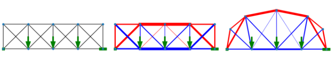
Fig 7. The initial truss. It’s calculated forces. The optimized truss.

Future work

Assigning forces

The biggest problem with this system is that using lstsq to assign forces minimizes the L2 norm of the forces when there are multiple possible solutions, which isn’t actually the “cheapest” possible solution! In theory, the cheapest truss could contain several very high forces, and many very small forces (imagine the pillars of a supension bridge.)

Dynamically change nodes and topology

It would be interesting to let the optimization dynamically add and remove nodes and edges in addition to just moving the nodes! I could imagine deleting any edges/nodes where the force goes to zero, and adding new nodes in the middle of high-force beams! It would also be fun to randomly initialize a truss and watch what it develops into.